Discrete connections (part V)

This part will deal mainly with the constructive elements of a fractal class derived from the conjectured asymptotic nature of the euclidean summation.
First some basic sequences and functions:

r-golden ratio builder

[;g_0^r=r, \; g_{n+1}^r = 1 + \frac{1}{g_n^r};]

upward shifted by r identity

[;u_n^r=n+r;]

upper ratio coefficient

[;\overline{\lambda}:[0,\infty) \rightarrow (0,1], \; \overline{\lambda}(x)=\frac{1}{1+x};]

where r>0 is a real number.

Let us consider some properties of the above sequences and functions:

[;\lim_{n\rightarrow \infty}\overline{\lambda}(g_n^r) = 1-\phi, \sum_n (-1)^n \cdot \prod_{i=0}^{n} \overline{\lambda}(g_i^r) \; convergent;]

[;\lim_{n \rightarrow \infty} \overline{\lambda}(u_n^r) = 0, \prod_n (1 - \overline{\lambda}(u_n^r)) \; convergent \; to \; 0;]

For the upward shifted by r identity, the conclusions are self evident due to:

[;\overline{\lambda}(u_n^r) = \frac{1}{1+n+r};]

and

[;\prod_{i=0}^{n} (1 - \overline{\lambda}(u_n^r)) = \frac{r}{1+n+r};]

For the r-golden ratio builder, the first conclusion's proof is based upon the relative positions of r and the golden ratio.

Indeed, if r is equal to the golden ratio then the r-golden ratio builder is stationary (and equal to the golden ratio).

From the two left cases let's consider the case r is smaller than the golden ratio. With this assumption we get:

[;r^2 -r -1 < 0 \Rightarrow g_1^r - g_0^r = -\frac{r^2-r-1}{r} > 0;] 

By means of mathematical induction one can prove that the subsequences of even index and odd index terms of the r-golden ratio are respectively increasing and decreasing. Since both sequences fall between the two first terms of the sequence results that they are both convergent to respectively g and h. 

We get successively:

[;\left\{ \begin{array}{rcl} g & = &1+\frac{1}{h}\\ h & = &1+\frac{1}{g} \end{array} \right. \Leftrightarrow \left\{ \begin{array}{rcl} g & = &1+\frac{1}{1+\frac{1}{g}} \\ h & = & 1+\frac{1}{g} \end{array} \right. \Leftrightarrow;]
[;\left\{ \begin{array}{rcl}g & = & \frac{2\cdot g +1}{g+1} \\ h & = & 1 + \frac{1}{g}\end{array}\right. \Leftrightarrow \left\{ \begin{array}{rcl} g^2 -g -1 & = & 0\\ h & = & 1 + \frac{1}{g} \end{array} \right. \Leftrightarrow;]
[;\left\{ \begin{array}{rcl}g & = & \varphi \\ h & = & 1 + \frac{1}{g}\end{array}\right. \Leftrightarrow \left\{ \begin{array}{rcl} g & = & \varphi \\ h & = & \varphi \end{array} \right.;]

Therefore the entire sequence is convergent to the golden ratio. Since the golden ratio is not equal to 1 results that:

[;\sum_n (-1)^n \cdot \prod_{i=0}^{n} \overline{\lambda}(g_i^r);]

is convergent.

Having these sequences and functions completely described let us consider the two mechanisms we will use in order to define the previously mentioned class of fractals:

The top value base sequence

For any four complex numbers u,v,w,z shaping a trapezoid and the sequences:

[;(\alpha_n)_{n\ge 0}, \; (\beta_n)_{n\ge 0};]

defined by:

[;\alpha_0=u, \; \beta_0=v, \beta_1=w,\; \alpha_1=z;]

and

[;\left\{ \begin{array}{rcl} \alpha_{n+2} & = & (1 - \overline{\lambda}(g_n^r))\cdot \alpha_{n+1}+ \overline{\lambda}(g_n^r) \cdot \alpha_{n} \\ \beta_{n+2} & = & (1 - \overline{\lambda}(g_n^r))\cdot \alpha_{n+1}+ \overline{\lambda}(g_n^r) \cdot \beta_{n} \end{array} \right. ;]

we have that:

[;(\alpha_n)_{n\ge 0} \rightarrow \alpha;]

The self-similarity base sequence

For any four complex numbers u,v,w,z shaping a trapezoid and the sequences:

[;(\tilde{\alpha}_n)_{n\ge 0}, \; (\tilde{\beta}_n)_{n\ge 0};]

defined by:

[;\tilde{\alpha}_0=u, \; \tilde{\beta}_0=v, \tilde{\beta}_1=w,\; \tilde{\alpha}_1=z;]

and

[;\left\{ \begin{array}{rcl} \tilde{\alpha}_{n+2} & = & (1 - \overline{\lambda}(u_n^r))\cdot \tilde{\alpha}_{n+1}+ \overline{\lambda}(u_n^r) \cdot \tilde{\alpha}_{0} \\ \tilde{\beta}_{n+2} & = & (1 - \overline{\lambda}(u_n^r))\cdot \tilde{\alpha}_{n+1}+ \overline{\lambda}(u_n^r) \cdot \tilde{\beta}_{0} \end{array} \right. ;]

we have that:

[;(\tilde{\alpha}_n)_{n\ge 0} \rightarrow \tilde{\alpha}_0;]

For both sequences r is the scaling ratio of the two parallel edges of the trapezoid i.e.:

[;(u-v)=r\cdot (z-w);]

The construction of the above two sets of sequences is better depicted by the following figures:

and

Next: The euclidean fractal class

Discrete connections (part IV)

Before dealing with the major results, let us consider the following:

 Intermediate recurrence

[;\frac{n}{2}<k<\frac{2\cdot n}{3} \Rightarrow;]

[;\tau_1(n,k)=k+\tau_1(n-k,2\cdot k - n);]

Its proof consists in applying the outer row recurrence first for n and k and then for k and n-k.

The first major result consists, as the above one, from two formula iterations:

Asymptotic expansion

a)

[;\frac{F_{2 \cdot m}}{F_{2 \cdot m + 1}} \cdot n <k< \frac{F_{2 \cdot m - 1}}{F_{2 \cdot m}} \cdot n \Rightarrow;]

[;\tau_1(n,k) = (\sum_{i=1}^{2 \cdot m - 1}(-1)^{i+1} \cdot F_{i}) \cdot n + (\sum_{j=2}^{2\cdot m} (-1)^{j+1} \cdot F_{j}) \cdot k +;]

[;\tau_1(F_{2 \cdot m-1} \cdot k - F_{2\cdot m - 2} \cdot n, F_{2 \cdot m - 1} \cdot n - F_{2 \cdot m} \cdot k);]

b)

[;\frac{F_{2 \cdot m}}{F_{2 \cdot m + 1}} \cdot n <k< \frac{F_{2 \cdot m + 1}}{F_{2 \cdot m + 2}} \cdot n \Rightarrow;]

[;\tau_1(n,k) = (\sum_{i=1}^{2 \cdot m }(-1)^{i+1} \cdot F_{i}) \cdot n + (\sum_{j=2}^{2\cdot m + 1} (-1)^{j+1} \cdot F_{j}) \cdot k +;]

[;\tau_1(F_{2 \cdot m - 1} \cdot n - F_{2 \cdot m} \cdot k, F_{2 \cdot m+1} \cdot k - F_{2\cdot m } \cdot n);]

where 

[;F_{1} = F_{2}=1;]

[;F_{m+2}=F_{m+1} + F_{m};] 

stand for the terms of the Fibonacci sequence, and by natural convention:

[;F_{0} = 0;]

The proof follows by mathematical induction, the base case being ensured by the outer row recurrence  (for a)) and the intermediate recurrence (for b)). For the inductive step we will suppose that a) and b) hold for n arbitrarily fixed m. Through the outer row recurrence results that a) holds for m+1 as well and in a similar fashion b) holds for m+1 as well, thus concluding the inductive reasoning.
Since from the previous part we have that:

[;\frac{\tau_2(n)}{n} < 1;]

and for a conveniently chosen m, via the asymptotic expansion we have that:

[;\frac{\tau_2(n)}{n} > \frac{F_{2\cdot m + 1} - 1}{ F_{2 \cdot m + 1}};]

we can now state that:

[;(\frac{\tau_2(n)}{n})_{n \ge 1} \rightarrow 1;]

There is also another gain (from the asymptotic expansion), from the perspective of the positional peak: if we squeeze k such that the fraction n/k becomes closer and closer to the golden ratio we get values of the euclidean summation pretty close to n. Alas we can only conjecture for now that:

[;(\frac{\tau_3(n)}{n})_{n \ge 1} \rightarrow \phi;]

where:

[;\phi = \frac{1}{\varphi} \approx 0.618;]

is called the golden ratio conjugate.

Next: Fractal candidate building blocks

Discrete connections (part III)

For the positional peak, its boundaries are straightforward (definition, inner row  recurrence and lower boundary):

[; \frac{n}{2}<\tau_3(n)<n \; \forall \; n \ge n_{\tau_3};]

For the peak, it's a two step argument. For the lower bound we consider two cases: n odd and respectively n even. For every such case we take a conveniently chosen pair, compute the euclidean summation and truncate it up to a suitable value:

 [; n = 2 \cdot k + 1 \Rightarrow ;]

[; \tau_1(n,k+2) = n-(k+2) + \tau_1(k+2, k-1) \Rightarrow ;]

[; \tau_1(n,k+2) \ge k-1 + 3= k+2 > k + \frac{1}{2} = \frac{n}{2} ;]

[; n=2\cdot k \Rightarrow ;]

[;\tau_1(n,k+1) = n-(k+1) + \tau_1(k+1, k-1) \Rightarrow ;]

[; \tau_1(n,k+1) \ge k-1 + 2= k+1 > k = \frac{n}{2};]

Here also the inequality holds from a rank on, due to the approximations used.

For the upper bound, our reasoning will follow the rules of the mathematical induction:

 base case

[;\tau_1(1,0)=0<1;]

inductive step (n arbitrarily fixed)

[;\tau_1(k,r)<r \; \forall \; k,r \; such \; that \; n>k>r \Rightarrow ;]

[;\forall \; k<n \Rightarrow \exists \; q,r \; such \; that \;q \ge 1, k>r, n=q\cdot k + r  \Rightarrow ;]

[;\tau_1(n,k) = r + \tau_1(k,r) < r + k \le r + q \cdot k = n;]

thus concluding our reasoning.

We get in conclusion:

[; \frac{n}{2}<\tau_2(n)<n \; \forall \; n \ge n_{\tau_2};]

Next: Asymptotic behaviors of peak and positional peak.

Discrete connections (part II)

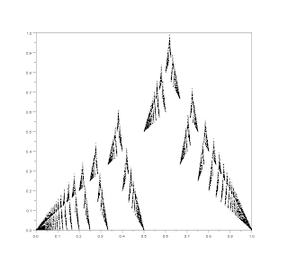
First, some Scilab-powered graphic suggesting the conjectured fractal nature of the euclidean summation:

The normalized euclidean summation (m=10000 and 0<n<10000)

But science relies upon facts, so let's begin by listing some of the basic properties of the euclidean summation:

Lower boundary

[;\tau_1(n,k) = 0 \Leftrightarrow (k=0)$ or $((k\neq 0)$ and $(k|n));]

Homogeneity

[;\tau_1(p\cdot n, p\cdot k) = p \cdot \tau_1(n,k);] 

Column periodicity

[;m_1\equiv m_2\pmod{n}$ $\Rightarrow$ $\tau_1(m_1, n) = \tau_1(m_2,n);]

Outer row recurrence

[;\frac{n}{2}<k<n \Rightarrow \tau_1(n,k) = n-k + \tau_1(k,n-k);]

Inner row recurrence

[;\frac{n}{2}<k<n \Rightarrow \tau_1(n,k) = n-k + \tau_1(n,n-k);]

Diagonal periodicity

[;\frac{n}{2}<k<n \; and \; 0 \le r < (n-k) \Rightarrow ;]

[;\tau_1(n + p \cdot (n-k) + r, k + p \cdot (n-k) + r) = \tau_1(n+r, k+r) ;]

Next: Boundaries for peak and positional peak

Discrete connections (part I)

As you probably expected, all the previous subjects (Fibonacci sequence, golden ratio and fractals) are the pieces of a larger puzzle: a set of mathematical tools describing the nature of numbers. Their connection comes from a rather unexpected place: the greatest common divisor (the largest number dividing both numbers) algorithm as described by Euclid.
The algorithm states that in order to compute the gcd of two natural numbers m and n it suffices to compute the quotient q and remainder r from their integer division, and if r is non-zero repeat the procedure for n and r. The last non-zero remainder obtained in this manner, or n if no such remainder existed, is the gcd.
The subject of the Euclid's algorithm was intensively studied throughout the history of mathematics, one of the most interesting results (involving also Fibonacci numbers) being Lamé's theorem describing the number of steps it takes to compute the gcd for a given pair or numbers a and b.
The novel (to be read independent, since I consider that most of the time we reinvent the math) approach considers a rather unexplored characteristic of the algorithm, that of the summation of the remainders.
Thus let us define the euclidean summation, euclidean summation peak and euclidean summation positional peak by the following:

[; \tau_{1}(m,n) = m\mod n + \tau_{1}(n, m\mod n) ;]
[; \tau_{2}(n)=\max\{\tau_{1}(n,k)| 0\le k \le n\};]
[; \tau_{3}(n) = \max \{k|0 \le k \le n \; and \; \tau_{1}(n,k)=\tau_2(n) \} ;]

where mod is the extended modulus operator of two natural numbers, i.e. the remainder of their integer division, if the divisor is non-zero and zero otherwise.
The purpose of this blog-based article is to conjecture (and maybe someday prove) the fractal nature of the sum of remainders, fully describe a strong candidate for it and some tools to describe the common properties of the two.
Hope you'll find it interesting enough to stop by every now and then for updates.

Fractals and life (part I)

Well, these are a special breed of mathematical beasts, they are ever growing collections of dots and no matter how deep you zoom them in you'll get about the same picture as you got when looking at the original.
As an example, one of the most intuitive ones, we will consider Sierpinski's triangle: let us take a triangle with all sides equal and join the middles of its sides. We thus get four smaller triangles. Lets cut off the one in the center. We now have only three triangles in the corners, and repeat for each one of them the same procedure: join middles and cut the center triangle. If we infinitely repeat the procedure we would obtain something that looks like this:

Where does life use these kind of tools? Frosted window patterns, broccoli, shattered compact discs, Scandinavian fjords and the list goes on. 

References:

Artwork: http://www.zeuscat.com/andrew/chaos/sierpinski.html

Examples: http://en.wikipedia.org/wiki/Main_Page

Golden ratio and life (part I)

Warning: Starting with this blog you may need some additional magic: in order to typeset mathematical formulas I used a script file named TeX THE WORLD. Consequently you may have to enable javascript in your browser (Greasemonkey and the same user script). Sorry about the inconvenience, but this way maths look better.

As it's name states, the golden ratio has everything to do with geometry and aesthetics. It was defined by the following property: "Given a line segment of length c, how can we divide it in two sub-segments of lengths a and b (c=a+b, a > b) such that the ratio of the large over the small equals the ratio of the segment over the large?" Otherwise said:

[; \varphi = \frac{a}{b} = \frac{c}{a} ;]

Now, replacing c by the sum of a and b, we get:

[; \varphi = \frac{1 + \varphi}{\varphi} ;]

hence:

 [; \varphi = \frac{1+\sqrt{5}}{2} \approx 1.618 ;]

This proportion was deeply engraved in ancient (the Parthenon), Renaissance (Mona Lisa) and modern (The Sacrament of the Last Supper) masterpieces of painters and architects, and all for a reason: mathematics ARE aesthetically pleasing.
And coincidences don't stop here: remember the Fibonacci sequence? Let's consider consecutive terms ratios and place them like this:

[;\frac{1}{1}, \frac{3}{2}, \frac{5}{8}, ... ? ... , \frac{13}{8},\frac{5}{3},\frac{2}{1};]

We get two sequences, an increasing one and a decreasing one, both leading to ... the golden ratio. So, if you want to use golden ratio-like proportions, the Fibonacci numbers are your best choice, no need for tedious square roots.

Fibonacci and life (part I)

I chose Fibonacci's sequence as a starting point of my blog for several reasons:

1. It's plain (no tricks);
2. It branches into our day-to-day living in surprising ways.

So let's give it a go: 1, 1, 2, 3, 5, 8, ... can you see the pattern? Yup! You got it, starting from 2 all the terms of the sequence are the sum of the previous two (1+1=2, 1+2=3, ...). Now where does real life kick in? You've all heard about the saying "breeding like rabbits", but never imagined the mathematical extents of it:

• first we buy a male rabbit and a female rabbit (no gender discrimination intended) (1 pair);
• the first month they have no baby rabbits (not mature enough) (1 pair);
• the second month they have two baby rabbits, a male and female (2 pairs);
• the third month the original pair has two more baby rabbits (male and female), their first babies are not mature yet so they have none (3 pairs); 
• the fourth month both the original pair and their first pair of babies (yeah, I know, they mate family, the animals!) have each one pair of babies (5 pairs);
• a.s.o. many, many rabbits.

Luckily for us there is such thing as natural selection through predators, disease or genetics and the math does not ensure rabbits' world domination.

Let there be science

Knowledge is power, so I decided to let it flow. Bare with me since this is the first of many. I will try to make it as scientific as it gets and be receptive to constructive criticism.